Motivation: Realtime Deployability

One of the main problems of our initial models for the Neural Decoding Task was the lack of realtime deployability. They use an input buffer window of 1024 steps, where each step represents 4 ms. This results in a total buffer window and a latency of 4.096 s. The models are executed for non-overlapping windows of size 1024, meaning that the model execution rate is 0.244 Hz. However, in theory the models had a high flexibility in the possible latency and execution rate that they could achieve, as both the convolutional and the recurrent layers allow for an iterative implementation.

The models used a kernel size of 3 applied in two convolutional blocks. The receptive field determined by this structure can be visualized below.

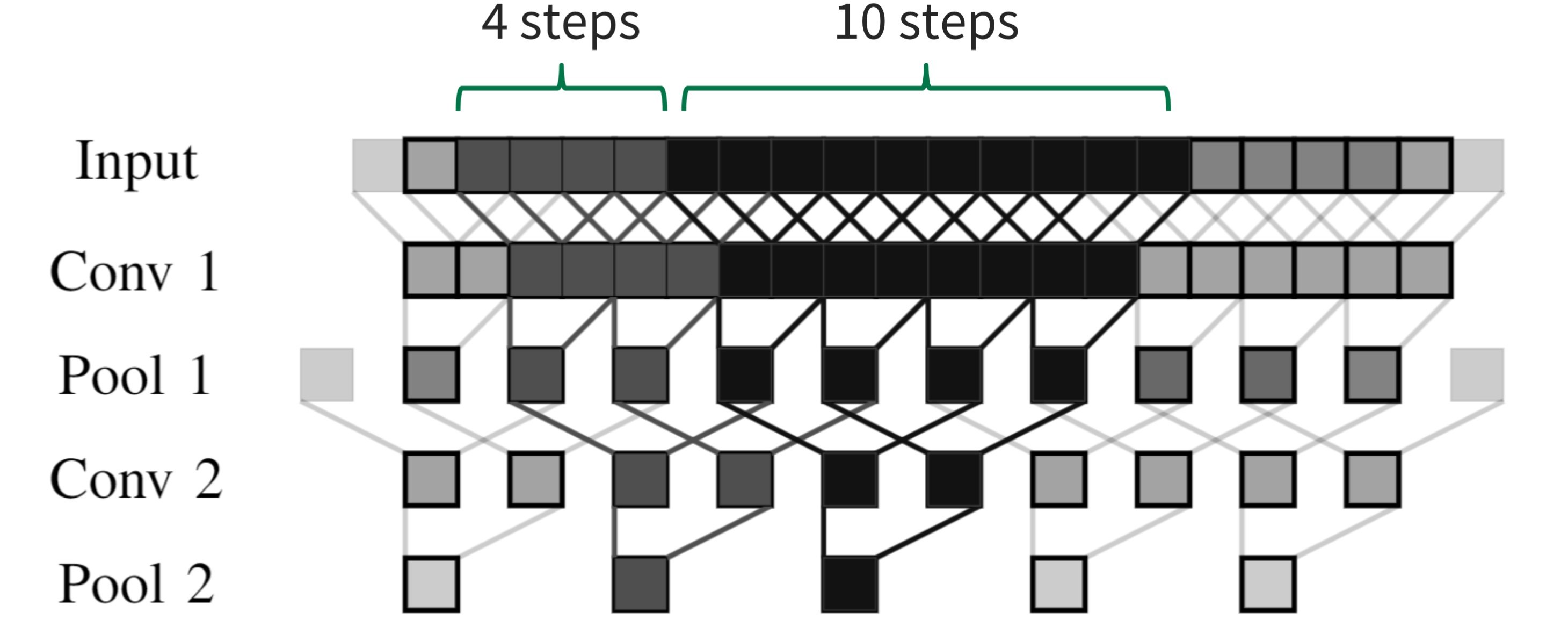
With the sizes mentioned above, the computation of one keypoint requires an effective buffer window of 10 steps, which offers a latency of 40 ms. This would also reduce the input buffer size from 1024 to 10. The stride of the receptive field is 4 steps, or 16 ms, which translates to an execution rate of 62.5 Hz. The theoretical upper limit of the latency of our models (40 ms) is well under the time delay between stimulus and voluntary muscle movement reported by the neuroscience literature, which is typically greater than 100 ms. Assuming no further latencies arise from signal transmission and ignoring computation time, our approach would be suitable for deployment in the real world, given an appropriate real-time implementation of the networks.

Realtime Convolutional Layers

We explore an iterative implementation of the architecture introduced before for maximizing the real-time applicability of the networks. For this, we compute the effective receptive field size in each convolutional and pooling layer required to compute one keypoint for each model (see Figure a).

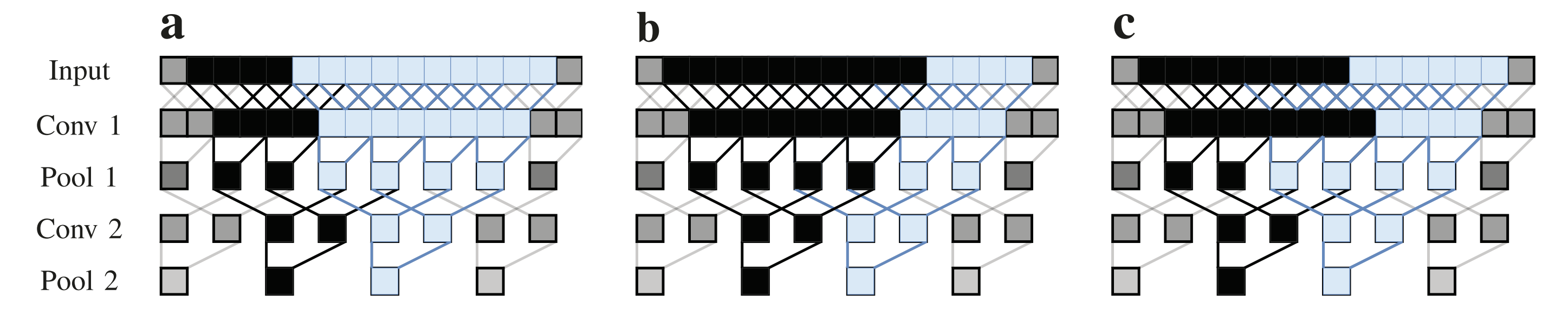
This is accomplished by working back from one keypoint and iteratively determining the size of the previous layer required to compute the output of a size represented by the receptive field of the current layer. The size determined by half of the buffer size of the initial layer + 1 step represents the model’s latency since the original model’s training is performed with centered kernels. In order to avoid repeating computations that have already been performed, for each layer’s buffer, we determine the size of the new data required to add to the current receptive field that allows the computation of a new keypoint (see Figure b). We then compute the size of the buffer needed to compute the new data in the next layer (see Figure c). These buffer sizes are used to implement the real-time version of the model.

Paper    YouTube   

BibTeX